An Experiment: the Cauchy–Schwarz inequality
[examples Archive of Formal Proofs analysis Isar The Cauchy–Schwarz inequality is a well-known fact about vector inner products. It comes in various forms that any mathematician is expected to recognise.
A successful search
During discussions with colleagues, the question came up: is Cauchy–Schwarz available in the Isabelle/HOL libraries? I got a quick answer, thanks to the SErAPIS search engine. I typed the phrase into the “concept” box and immediately got several close hits. (It helps that the theorem names actually match!)
lemma Cauchy_Schwarz_ineq:
  "(inner x y)⇧2 ≤ inner x x * inner y y"
proof (cases)
  assume "y = 0"
  thus ?thesis by simp
next
  assume y: "y ≠ 0"
  let ?r = "inner x y / inner y y"
  have "0 ≤ inner (x - scaleR ?r y) (x - scaleR ?r y)"
    by (rule inner_ge_zero)
  also have "… = inner x x - inner y x * ?r"
    by (simp add: inner_diff)
  also have "… = inner x x - (inner x y)⇧2 / inner y y"
    by (simp add: power2_eq_square inner_commute)
  finally have "0 ≤ inner x x - (inner x y)⇧2 / inner y y" .
  hence "(inner x y)⇧2 / inner y y ≤ inner x x"
    by (simp add: le_diff_eq)
  thus "(inner x y)⇧2 ≤ inner x x * inner y y"
    by (simp add: pos_divide_le_eq y)
qed
This version is a close match to the Wikipedia description and to the abstract formulation, namely
\[\mid\langle \mathbf{u},\mathbf{v} \rangle{\mid}^2 \le \langle \mathbf{u},\mathbf{u}\rangle \langle \mathbf{v},\mathbf{v}\rangle.\]Unfortunately, this abstract version––for the Isabelle type class real_inner of real inner product spaces––is not easily related to the concrete version with explicit summations, which is what I wanted. Such special cases look quite different from the abstract version, and even Wikipedia enumerates them separately.
Googling around for a simple concrete proof took me to Hölder’s inequality, which follows from Young’s inequality for products, which holds “because the logarithm function is concave”, which is a special case of Jensen’s inequality.
A rabbit hole of inequalities!
Concave and convex functions
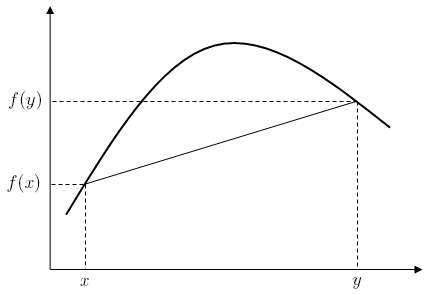
The following diagram (borrowed from Wikipedia) shows what a concave function looks like.
And a concave function is the negation of a convex function. Turning to SErAPIS again, I discovered that both concepts were defined in Isabelle’s Archive of Formal Proofs (AFP). Moreover, convex functions were defined in the Isabelle libraries themselves, along with the key property that a function is convex if its second derivative is nonnegative.
So by including the library session HOL-Analysis, concave functions are trivial to define:
definition concave_on :: "'a::real_vector set ⇒ ('a ⇒ real) ⇒ bool"
  where "concave_on S f ≡ convex_on S (λx. - f x)"
Their characteristic inequality follows by simply negating the inequality for convex functions:
lemma concave_on_iff:
  "concave_on S f ⟷
    (∀x∈S. ∀y∈S. ∀u≥0. ∀v≥0. u + v = 1 ⟶ f (u *⇩R x + v *⇩R y) ≥ u * f x + v * f y)"
  by (auto simp: concave_on_def convex_on_def algebra_simps)
Recall that Young’s inequality requires proving that the logarithm function is concave (on the positive reals). The Isabelle proof loois like this:
lemma ln_concave: "concave_on {0<..} ln"
  unfolding concave_on_def
  by (rule f''_ge0_imp_convex derivative_eq_intros | simp)+
A little magic is happening here. After we unfold the definition of concave, the first step is to invoke the theorem f''_ge0_imp_convex, giving sufficient conditions for a function to be convex. There are four:
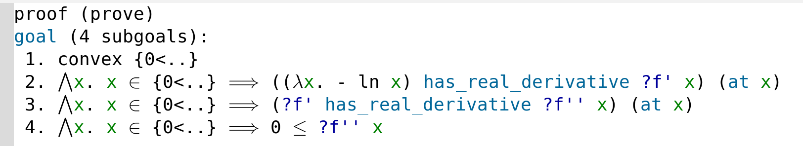
Let’s express these formulas in plain language:
- The set of positive real numbers (written as
{0<..}) is a convex set. This will be proved automatically thanks to some library theorem about intervals. - The negation of the logarithm ($\lambda x. - {\ln x}$) has some derivative, written as
?f' x. The question mark indicates a unifiable variable or unknown, which needs to be replaced by the actual derivative. It can depend uponx, which is a positive real. - The function
?f'has some derivative, written as?f'' x. This is the second derivative. - This second derivative is nonnegative for all positive reals.
Proving these subgoals involves discovering the first derivative and then the second and finally proving the second to be nonnegative. One might imagine a lot of work to be necessary, but the magic line
(rule derivative_eq_intros | simp)+
is sufficient to calculate and simplify the derivative even of many complicated formulas.
Since the proof method rule can be given any number of lemmas or inference rules to try, we can throw in f''_ge0_imp_convex as well, yielding the two-line proof of ln_concave shown above. That result immediately allows us to prove one formulation of Young’s inequality, $a^\alpha b^\beta \le \alpha a + \beta b$ where $\alpha+\beta=1$:
lemma Youngs_inequality_0:
  fixes a::real
  assumes "0 ≤ α" "0 ≤ β" "α+β = 1" "a>0" "b>0"
  shows "a powr α * b powr β ≤ α*a + β*b"
proof -
  have "α * ln a + β * ln b ≤ ln (α * a + β * b)"
    using assms ln_concave by (simp add: concave_on_iff)
  moreover have "0 < α * a + β * b"
    using assms by (smt (verit) mult_pos_pos split_mult_pos_le)
  ultimately show ?thesis
    using assms by (simp add: powr_def mult_exp_exp flip: ln_ge_iff)
qed
A more standard formulation, $ab\le a^p/p + b^q/q$ where $1/p+1/q=1$, holds by a suitable substitution into the previous result:
lemma Youngs_inequality:
  fixes p::real
  assumes "p>1" "q>1" "1/p + 1/q = 1" "a≥0" "b≥0"
  shows "a * b ≤ a powr p / p + b powr q / q"
proof (cases "a=0 ∨ b=0")
  case False
  then show ?thesis
  using Youngs_inequality_0 [of "1/p" "1/q" "a powr p" "b powr q"] assms
  by (simp add: powr_powr)
qed (use assms in auto)
But having got this far, I felt rather lazy (it was a Saturday) and instead of trying to prove Hölder’s inequality I asked what would happen if I took the proof about inner products at the top of this page and substituted the obvious summation over a fixed index set. And here is the result, with almost no effort:
lemma Cauchy_Schwarz_ineq_sum:
  fixes a :: "'a ⇒ 'b::linordered_field"
  shows "(∑i∈I. a i * b i)⇧2 ≤ (∑i∈I. (a i)⇧2) * (∑i∈I. (b i)⇧2)"
proof (cases "(∑i∈I. (b i)⇧2) > 0")
  case False
  then consider "⋀i. i∈I ⟹ b i = 0" | "infinite I"
    by (metis (mono_tags, lifting) sum_pos2 zero_le_power2 zero_less_power2)
  thus ?thesis
    by fastforce
next
  case True
  define r where "r ≡ (∑i∈I. a i * b i) / (∑i∈I. (b i)⇧2)"
  with True have *: "(∑i∈I. a i * b i) = r * (∑i∈I. (b i)⇧2)"
    by simp
  have "0 ≤ (∑i∈I. (a i - r * b i)⇧2)"
    by (meson sum_nonneg zero_le_power2)
  also have "… = (∑i∈I. (a i)⇧2) - 2 * r * (∑i∈I. a i * b i) + r⇧2 * (∑i∈I. (b i)⇧2)"
    by (simp add: algebra_simps power2_eq_square sum_distrib_left flip: sum.distrib)
  also have "… = (∑i∈I. (a i)⇧2) - (∑i∈I. a i * b i) * r"
    by (simp add: * power2_eq_square)
  also have "… = (∑i∈I. (a i)⇧2) - ((∑i∈I. a i * b i))⇧2 / (∑i∈I. (b i)⇧2)"
    by (simp add: r_def power2_eq_square)
  finally have "0 ≤ (∑i∈I. (a i)⇧2) - ((∑i∈I. a i * b i))⇧2 / (∑i∈I. (b i)⇧2)" .
  hence "((∑i∈I. a i * b i))⇧2 / (∑i∈I. (b i)⇧2) ≤ (∑i∈I. (a i)⇧2)"
    by (simp add: le_diff_eq)
  thus "((∑i∈I. a i * b i))⇧2 ≤ (∑i∈I. (a i)⇧2) * (∑i∈I. (b i)⇧2)"
    by (simp add: pos_divide_le_eq True)
qed
That’s the great thing about structured proofs: they can easily be modified to prove related results. There may well be a clever way to prove this fact from Cauchy_Schwarz_ineq by unfolding the function inner, which has multiple definitions (one for each instance of the real_inner type class). But sometimes, simplest is best.
Note: all of the material above is scheduled for inclusion in the next Isabelle release, planned for December 2021. It can also be downloaded.
Exercises
It’s worth practising the derivative trick mentioned above. Here I have introduced the dummy predicate P in order that the proof will fail, allowing you to see what derivative was computed. You should be able to guess the derivative of the last example without running it. Note the use of the rules exI and conjI to strip off the outer connectives.
lemma "∃f'. ((λx. x^3 + x⇧2) has_real_derivative f' x) (at x) ∧ P (λx. f' x)"
  apply (rule exI conjI derivative_eq_intros | simp)+
lemma "x > 0 ⟹ ∃f'. ((λx. (x⇧2 - 1) * ln x) has_real_derivative f' x) (at x) ∧ P (λx. f' x)"
  apply (rule exI conjI derivative_eq_intros | simp)+
lemma "∃f'. ((λx. (sin x)⇧2 + (cos x)⇧2) has_real_derivative f' x) (at x) ∧ P (λx. f' x)"
  apply (rule exI conjI derivative_eq_intros | simp)+
If you have ever written code in Prolog to calculate symbolic derivatives, you’ll understand what’s going on here.