Machine Logic

Martin-Löf type theory in Isabelle: examples

30 Nov 2022

The previous post describes the implementation of Martin-Löf type theory in Isabelle. The ability to enter the rules in a notation as close as possible to the original papers and use them immediately for proofs was one of my key objectives for Isabelle in the 1980s. Now, through some tiny examples, let’s see how terms can be built incrementally with the help of schematic variables and higher-order unification. Such terms can be proof objects, but they do not have to be.

Incremental term construction

The simplest possible example is to use the type formation rules, available as form_rls, a list of theorems starting with those for $N$ and the $\Pi$-types. In this way we can enumerate well-formed types by generating the corresponding proofs.

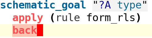
To begin, we enter a schematic goal. This allows the use of schematic variables in the goal, presumably with the expectation that they will be replaced during the course of the proof. Isabelle displays these instantiations.

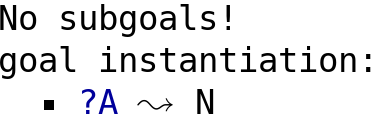
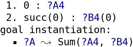
Our initial goal invites Isabelle to generate a well formed type in any possible way:

The cursor is placed after the application of the typing rules, which have instantiated ?A with the type N:

We have the option of asking Isabelle to backtrack over its most recent choice. Prolog programmers will notice the similarity to rejecting a Prolog output by typing a semicolon:

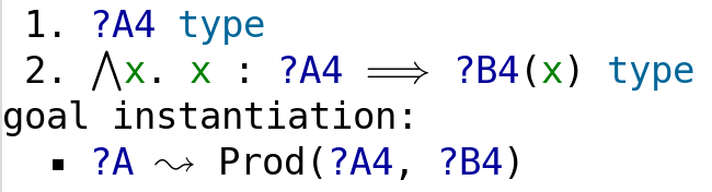
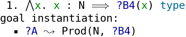
Backtracking has taken us to the next type formation in the list, which is for $\Pi$-types. But now we are required to synthesise two additional types ?A4 and the indexed family ?B4(x):

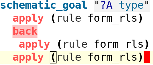
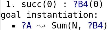
We continue by applying the same list of type formation rules again:

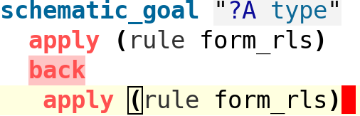
The obvious choice for ?A4 is once again N. Note how type ?A below is now partially filled in:

We unimaginatively continue with the same set of rules, to instantiate the last remaining type.

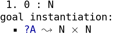
The family of types ?B4(x) has been instantiated (yet again) with N. It is a degenerate family with no dependence on x.

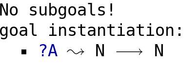
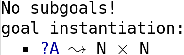
So the $\Pi$-type degenerates to a mere function type and is displayed as such, thanks to some syntactic trickery in the implementation of CTT. We could have continued to backtrack in order to generate other well-formed types.

Explicit backtracking, such as is shown here, is provided so that people can explore the proof space and sketch the design of backtracking-based proof automation. However, it should never form part of a polished proof because the reader has no chance of following what is going on.

Type inference

Type inference means to deduce the type of a given expression. It’s not always well-defined: some expressions will not have any type, which implies they are meaningless. On the other hand, $\lambda x.\,x$ can have any type of the form $A\to A$ where $A$ is a well-formed type.

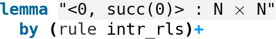
Let us deduce the type of the ordered pair $\langle 0,1\rangle$. It will suffice to use the introduction rules, which are bound to the name intr_rls. We once again enter a schematic goal, with a schematic variable where the expected type should go. Proving the theorem will fill in this type.

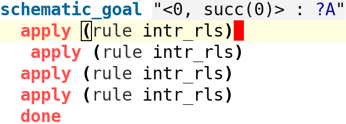
The first application of intr_rls will find the only possible match, namely the introduction rule (called SumI) for a ∑-type. The two subgoals demand type inference for the terms 0 and succ(0). The type of the second component is allowed to depend on the value of the first.

For each successive application of intr_rls, the cursor moves down. Let’s look at the corresponding outputs. After the second step, the term 0 has been given type N and the corresponding subgoal has disappeared. The type of the entire expression, given by the schematic variable ?A, has been updated accordingly.

After the third step, because of the succ function, the type of the second component is also seen to be N. There is no dependence, and the degenerate ∑-type is now displayed as simply N×N. Isabelle relies on syntactic trickery to achieve this.

The fourth and final step solves the remaining subgoal. This is only possible because 0 also has type N; an ordered pair in this position would have prevented this step and of course the corresponding term would be nonsensical.

That was straightforward but the proof is too long, especially as it’s so repetitious. Even in 1986, we could automate that sort of thing. Here is the exact same proof, but this time declared as an ordinary lemma (these don’t allow schematic variables, so the type is already filled in) and with the proof done by repetition.

Type inference of the addition function

The following example is much more complicated. Addition of natural numbers is expressed using the eliminator for type N, which is a higher order primitive recursion combinator. Type inference here requires inferring the types of the zero and successor cases, which need to be the same, well-formed type. The task requires many steps, but they are routine and can be performed by a mindless repetition of the type formation, introduction and elimination rules.

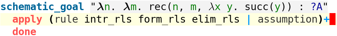
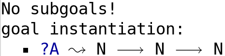
In this case, two Π-types are inferred (thanks to the use of λ), but has there is no actual dependence, they degenerate to a function type:

Watching proof objects emerge

A key selling point of Martin-Löf type theory in the 1980s, at least to me, was that you got a proof object (a “construction”) every time you proved a theorem (“type inhabitation”). Under the propositions-as-types interpretation, the type $A\times A\to A$ corresponds to the tautology $A\land A\to A$:

The proof above also uses repetition of the type formation, introduction and elimination rules, but on this occasion with the special proof method erule for the elimination rules. We need to take more care when generating, rather than typing, proof objects.

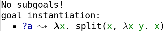
The proof method solves the goal and instantiates the schematic variable ?a with a proof object involving the Σ-type eliminator, split. We have synthesised the function to return the first component of an ordered pair.

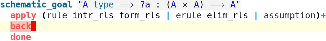
What’s cool is that if we reject this solution by backtracking, we get instead the function to return the second component of an ordered pair (compare $\lambda x\,y.\,x$ and $\lambda x\,y.\,y$).

Structured proofs in constructive type theory

As far as I can tell, nobody in the type theory world took the slightest interest in this implementation. I gave it up as a bad job. The material distributed with Isabelle represents work that is 30 years old. However, those CTT experiments were the starting point of all the automation provided now for Isabelle/ZF and Isabelle/HOL.

Isabelle continued to evolve, and along the way, the Isar language was introduced (by Makarius Wenzel). Since Isabelle is generic, improvements to the core system are inherited to all the logic instantiations. We get, for free, the ability to write structured Isar proofs in constructive type theory.

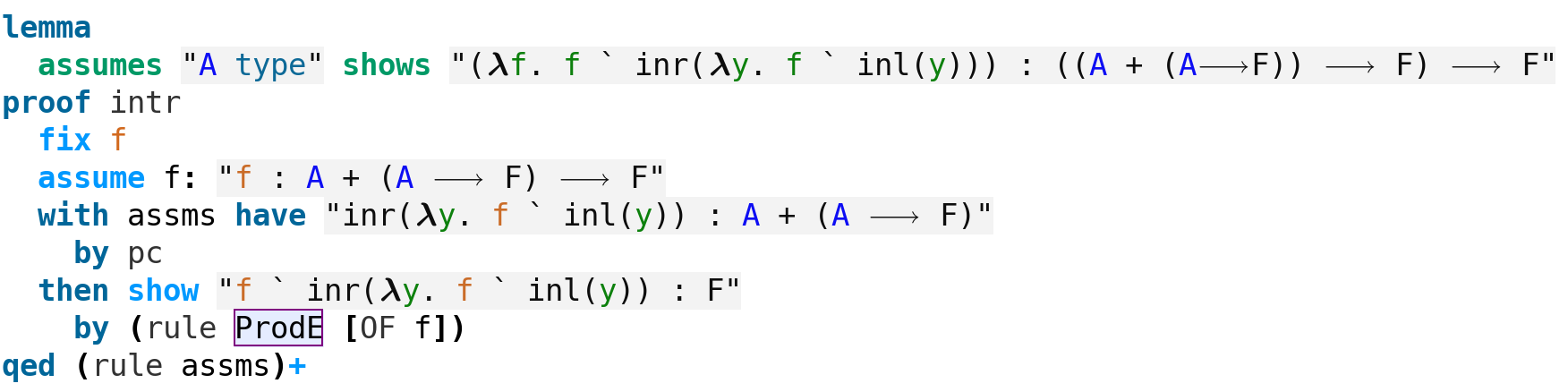
The double negation of the excluded middle

As everybody knows, the law of the excluded middle fails constructively. However, its double negation is an intuitionistic tautology. If $\neg(A\lor\neg A)$ then (since it implies $\neg A$) we obtain $A\lor\neg A$, a contradiction. This proof should be evident in the structured proof below:

The axiom of choice

Martin-Löf gave a derivation of the axiom of choice as his sole example when he published his type theory.¹ Although his proof is detailed, including the construction of the corresponding proof object, It was tricky to push through Isabelle. In the structured proof shown below, some echoes of his proof can be seen. This version, however, takes the proof object as given. It’s possible to write a line by line proof from which this object emerges.

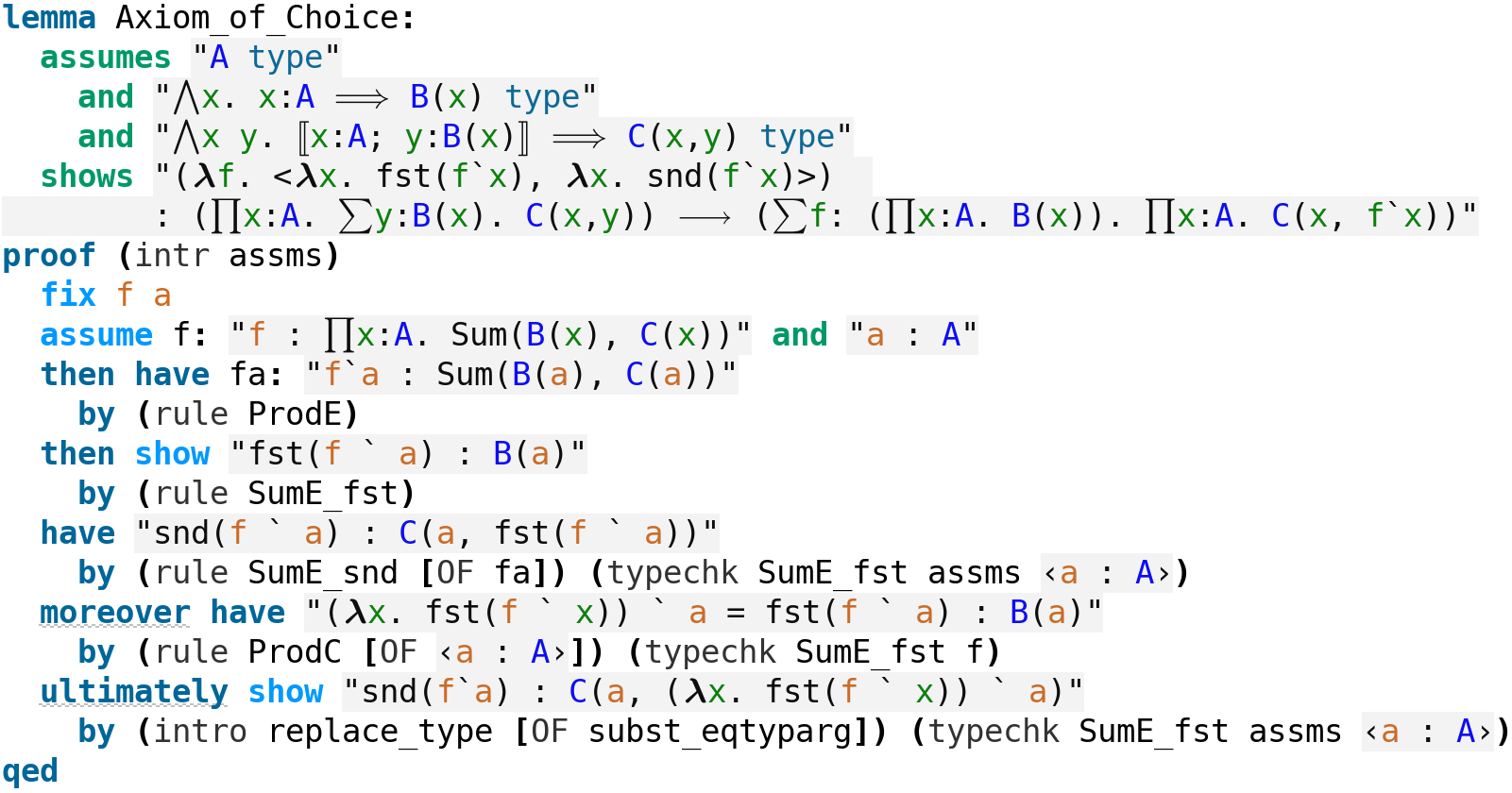
I recall being told that the Isabelle/CTT formalisation was not faithful because the variables in contexts were bound when they were not bound variables in the writings of Martin-Löf. I can only imagine that the proof above will be viewed by some with horror. And yet the one derivation he himself supplied in that paper does not show a single context. It looks quite a bit like the machine proof above.

Final remarks

The CTT development contains both the Martin-Löf type theory rules presented in the previous post and a tiny development of elementary arithmetic: addition, multiplication, division and remainder. You can download the examples in this post (plus others).