Definite integrals, I: easy cases over finite intervals
[examples formalised mathematics Isar analysis On occasion, your Isabelle proof may require you to work with a definite integral. (That is, the area under a curve between two points on the x-axis.) In the simplest case, all we have to do is integrate the given function to obtain its antiderivative, which we then evaluate at the endpoints, returning the difference. But things are not always simple. There could be discontinuities in the integrand (the function being integrated) or in its antiderivative. Either or both of the endpoints could be infinite. And while we say “area under a curve”, our notion of area is in fact signed, going negative when the curve crosses the x-axis. Finally, Isabelle has no actual capability to take integrals. Let’s work through a few examples in which we symbolically evaluate a definite integral, proving that the result is correct.
A baby example
Let’s begin with the following integral:
\[\begin{equation*} \int_{-1}^1 \frac{1}{\sqrt{1-x^2}}\, dx = \pi \end{equation*}\]Here is a graph of the integrand. It goes to infinity at both endpoints. Still, the integral is defined.
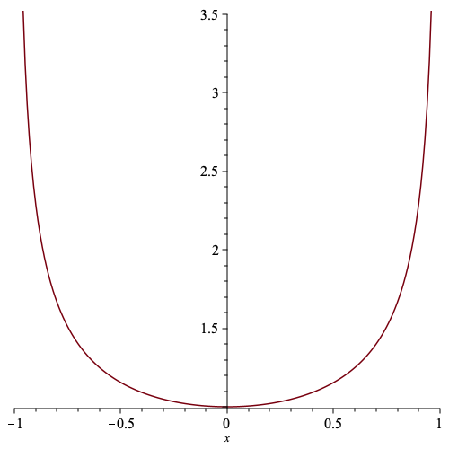
The antiderivative is $\sin^{-1}$, the inverse sine function, which is continuous. The integral is $\sin^{-1}(1) - \sin^{-1}(-1) = \frac{\pi}{2} - (-\frac{\pi}{2}) = \pi$.
To do this in Isabelle, our first task is to carry out the integration. Isabelle has no such capability, but that doesn’t matter: Isabelle can differentiate, so we simply use some external tool to integrate, confirming its answer by formally proving that its derivative matches the original integrand. This is an appeal to the Fundamental Theorem of Calculus (FTC), which says that integration and differentiation are inverse operations of each other. The Isabelle libraries provide numerous variants of this fact.
As for the external tool: WolframAlpha, which is free, can often do the job, but here I needed Maple to find out that the antiderivative was simply the inverse sine.
The Isabelle proof is so simple, there is almost nothing to say.
The key point is the form of the FTC chosen: fundamental_theorem_of_calculus_interior,
which allows the integrand to diverge at the endpoints provided the antiderivative is continuous over the full closed interval.
lemma "((λx. 1 / sqrt(1-x⇧2)) has_integral pi) {-1..1}"
proof -
  have "(arcsin has_real_derivative 1 / sqrt (1-x⇧2)) (at x)"
    if "- 1 < x" "x < 1" for x
    by (rule refl derivative_eq_intros | use that in ‹simp add: divide_simps›)+
  then show ?thesis
    using fundamental_theorem_of_calculus_interior [OF _ continuous_on_arcsin']
    by (auto simp: has_real_derivative_iff_has_vector_derivative)
qed
The proof begins by showing that the derivative of $\sin^{-1}$ is indeed $\frac{1}{\sqrt{1-x^2}}$, though only on the open interval $({-1},1)$. This fact, along with the continuity of $\sin^{-1}$, is supplied to the FTC, which sets up the calculation of $\sin^{-1}(1) - \sin^{-1}(-1)$.
A just slightly harder example
This next example, $\int_0^1 \frac{1}{\sqrt{x}}\, dx = 2$, presents the same difficulty: divergence at an endpoint.

Mathematically, its treatment is identical to the previous example. The integrand diverges at zero. Its antiderivative is $2\sqrt{x}$, which fortunately is continuous for all $x\ge0$.
As for the formal proof,
we use a little Isar to introduce the abbreviation f for the antiderivative,
which is referred to a number of times.
We prove that f is continuous over the closed interval and verify
that it has the correct derivative over the open interval,
avoiding the discontinuity at zero.
lemma "((λx. 1 / sqrt x) has_integral 2) {0..1}"
proof -
  define f where "f ≡ λx. 2 * sqrt x"
  have "(f has_real_derivative 1 / sqrt x) (at x)"
    if "0 < x" "x < 1" for x
    unfolding f_def
    by (rule refl derivative_eq_intros | use that in ‹simp add: divide_simps›)+
  moreover
  have "continuous_on {0..1} f"
    by (simp add: continuous_on_mult continuous_on_real_sqrt f_def)
  ultimately
  have "((λx. 1 / sqrt x) has_integral (f 1 - f 0)) {0..1}"
    by (intro fundamental_theorem_of_calculus_interior)
       (auto simp: has_real_derivative_iff_has_vector_derivative)
  then show ?thesis
    by (auto simp: f_def)
qed
If the integrand is differentiable over the closed interval,
then the proof can be done using fundamental_theorem_of_calculus,
a version of the FTC that does not require a separate proof of continuity.
Taking derivatives in Isabelle
It’s easy to take the derivative of a function or to prove that it is continuous. Isabelle does not provide dedicated proof methods for such tasks, relying instead on its own Prolog-like proof engine. Above we used the following line, although variations are possible:
by (rule refl derivative_eq_intros | use that in ‹simp add: divide_simps›)+
Key is the theorem list derivative_eq_intros, which as of today has more than 140 entries.
A typical one says in essence that to show that the derivative of $\lambda x. f (x) + g(x)$ is $h$, show the following:
- that the derivative of $f$ is some $f’$,
- that the derivative of $g$ is some $g’$,
- that $(\lambda x. f’ (x) + g’(x)) = h$.
The point is that both $f’$ and $g’$ will be logical variables (in the Prolog sense),
so the repetitive application of derivative_eq_intros can calculate the derivatives of the subterms into them. We alternate with simplifier calls because the result of the raw process produces terms like $0\cdot x^1 + 1\cdot x^0$. But if the simplifier alters the outer form of the equations, say by moving a term across the equals sign, then the process probably won’t work. A little tinkering is sometimes necessary.
To prove that a function is continuous, use the theorem list continuous_intros.
The idea is similar to differentiation: in fact a lot simpler,
because there is nothing to calculate.
Therefore there is no need to call the simplifier.
We shall see several continuity proofs in the forthcoming Part II.