The Dottie Number
[examples Isar AI locales Archive of Formal Proofs Once upon a time, goes the story, a lady named Dottie got bored and started playing with her calculator, pressing the cosine key over and over again. At first the numbers fluctuated wildly, but over time they always settled down to approximately 0.739085. (This only works if your calculator is set to radians, not degrees.) She had discovered the unique fixed point of the cosine function. The Dottie number has several further properties: it is a global attractor, meaning the limit is the same no matter what number you start with, and it is transcendental. It is a great example for showing off a range of computer algebra techniques in Isabelle, such as differentiation and unlimited precision real computations. Let’s prove those properties just mentioned and calculate (by proof!) its value to 12 decimal places.
Getting started
We begin by defining dottie to be the unique fixed point of cos.
But this definition, using the definite descriptor THE, will be good for nothing
until both existence and uniqueness of a fixed point have been proved.
definition dottie :: real where
  "dottie ≡ THE x. cos x = x"
Those claims will be proved with the help of the function $g(x)=\cos x - x$. Note that it slopes downwards.
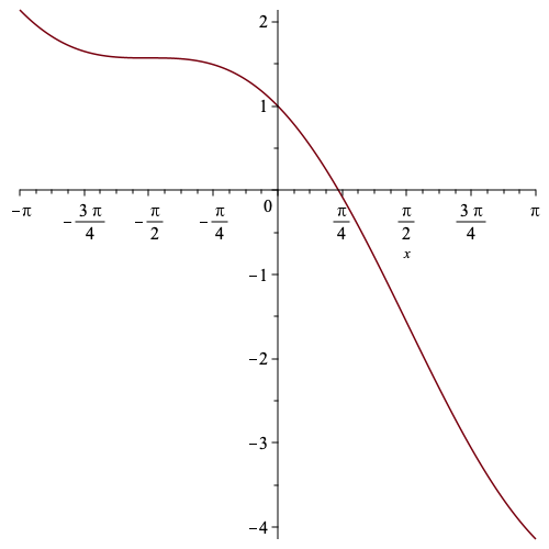
We can see that it has a unique root near $\frac{\pi}{4}$, but now we have to prove it. Several different theorems need facts about $g$, so to avoid duplication we create a locale where we can work with $g$.
locale Dottie =
  fixes g :: "real ⇒ real"
  defines "g ≡ λx::real. cos x - x"

begin
Thanks to the begin, we are now working inside the locale.
We have access to the function $g$ and can accumulate facts about it.
Our first task is to investigate its derivative.
lemma g_has_negative_deriv:
  assumes "¦t¦ ≤ 1"
  shows "∃d. (g has_real_derivative d) (at t) ∧ d < 0"
proof (intro exI conjI)
  show "(g has_real_derivative (- sin t - 1)) (at t)"
    unfolding g_def by (auto intro!: derivative_eq_intros)
  show "- sin t - 1 < 0"
    using assms pi_gt3 le_arcsin_iff [of _ t] by fastforce
qed
Isabelle is capable of calculating derivatives automatically.
The trick, as we see above, is to hit the goal repeatedly with derivative_eq_intros,
which is a collection of facts about derivatives of various operators.
The effect is practically the same as the schoolbook method.
If you know the derivative already, as here, it makes things easier to mention it.
Here we prove that the derivative of $g(t)$, which is $-\sin t-1$,
is strictly negative over the given interval $[-1,1]$.
Although computer algebra systems are not always sound, we can use them to write correct Isabelle proofs. Via the fundamental theorem of calculus, we can handle tough integrals. We give the hard work to the computer algebra system; Isabelle merely has to take the derivative of the claimed integral and compare that with the original integrand.
Existence
Existence is proved using the intermediate value theorem, which states that a function $g$ that is continuous on a given closed interval $[a,b]$ attains all the points between $g(a)$ and $g(b)$. Our $g$ is continuous. Since $g(0) = 1$ and $g(1) = \cos 1 - 1 < 0$, the IVT yields a point $x \in (0, 1)$ where $g(x) = 0$, which implies $\cos x = x$.
lemma dottie_exists: "∃x::real. 0 < x ∧ x < 1 ∧ cos x = x"
proof -
  have g_cont: "continuous_on {0..1} g"
    unfolding g_def by (intro continuous_intros)
  obtain "g 0 = 1" "g 1 < 0" using cos_1_lt_1 by (simp add: g_def)
  with IVT2'[of g 1 0 0] g_cont
  obtain x where hx: "0 ≤ x" "x ≤ 1" "g x = 0"
    by (metis less_eq_real_def zero_le_one)
  hence cos_eq: "cos x = x" by (simp add: g_def)
  with hx show ?thesis
    by (metis cos_1_lt_1 cos_zero order_less_le)
qed
In the proof above, we see a trick for proving continuity.
It resembles the trick for taking derivatives,
only we hit the goal with a different list of theorems, namely continuous_intros.
Then we show the $g$ crosses 0 to prove the existence of a fixed point
satisfying $0<x<1$.
Uniqueness
We proved above that the derivative of $g(x) = \cos x - x$ is strictly negative for $x \in [-1,1]$, i.e. $g$ is strictly decreasing, so $g$ can have at most one zero on that interval. And since $[-1,1]$, is the range of the cosine function, uniqueness over the entire real line immediately follows.
lemma dottie_unique:
  fixes x y :: real
  assumes "cos x = x" "cos y = y"
  shows "x = y"
proof (rule ccontr)
  assume "x ≠ y"
  have gx: "g x = 0" and gy: "g y = 0" using assms by (auto simp: g_def)
  show False
  proof (cases "¦x¦ > 1 ∨ ¦y¦ > 1")
    case True
    then show ?thesis
      by (metis assms abs_cos_le_one not_less)
  next
    case False
    then have "¦x¦ ≤ 1 ∧ ¦y¦ ≤ 1"
      by simp
    moreover have "x < y ∨ y < x" using ‹x ≠ y› by linarith
    ultimately show ?thesis
      using DERIV_neg_imp_decreasing [OF _ g_has_negative_deriv] gx gy
      by force
  qed
qed
More precisely, given the two claimed fixed points, $x$ and $y$, we first trivially establish that both must lie within the interval $[-1,1]$. Then, assuming for contradiction that $x\not=y$, one must be less than the other. So $g(x)<g(y)$ or $g(y)<g(x)$, because the derivative is strictly negative, but we know $g(x) = g(y) = 0$.
Approximating its value
This is a good example of using untrusted sources, such as a calculator, and validating them by formal proof to get an accurate approximation to Dottie.
definition lb::real where "lb ≡ 0.739085133215"
definition ub::real where "ub ≡ 0.739085133216"
Knowing that the function $g$ is strictly decreasing,
we can determine whether a given estimate is a lower bound or an upper bound.
We use the approximation proof method, which is based on interval arithmetic to investigate the ordering relationships.
lemma lb_gt: "cos lb > lb"
  unfolding lb_def by (approximation 50)

lemma ub_lt: "cos ub < ub"
  unfolding ub_def by (approximation 50)
Now we can prove that lb is a lower bound, by contradiction and monotonicity reasoning.
lemma lb: "lb < dottie"
proof (rule ccontr)
  assume neg: "¬ lb < dottie"
  have gd: "g lb > 0"
    using facts lb_gt by (auto simp: g_def)
  show False
    using DERIV_neg_imp_decreasing [OF _ g_has_negative_deriv] facts neg
    by (smt (verit, ccfv_SIG) cos_le_one cos_monotone_0_pi lb_gt pi_gt3)
qed
And analogously, ub is an upper bound.
lemma ub: "ub > dottie"
proof (rule ccontr)
  assume neg: "¬ ub > dottie"
  have gd: "g ub < 0"
    using facts ub_lt by (auto simp: g_def)
  show False
    using DERIV_neg_imp_decreasing [OF _ g_has_negative_deriv] facts neg
    by (smt (verit) cos_ge_minus_one ub_lt gd g_def)
qed
We have pinned down the Dottie number to 12 decimal places.
Something trivial
All this time, we were continuing to work in the locale because we needed
the lemma that the derivative of $g$ is negative.
But now, we are finished with $g$ and leave the locale.
We can refer to facts proved inside the locale using the prefix Dottie.
end
Since $\cos(\mathit{dottie}) = \mathit{dottie}$ and $\mathit{dottie} \in (0,1)$, and since $\sin^2 x+cos^2x = 1$, we easily get $\sin(\mathit{dottie}) = \sqrt{1 - \mathit{dottie}^2}$. Sledgehammer found this proof automatically.
lemma sin_dottie: "sin dottie = sqrt (1 - dottie⇧2)"
  by (smt (verit) Dottie.facts pi_gt3 sin_cos_sqrt sin_ge_zero)
The cosine function is a contraction map
The next step is to investigate why iterates of the cosine function always converge to the Dottie number. It’s because $\cos$ is a contraction on $[-1,1]$ with Lipschitz constant $\sin 1$, or with less jargon, $\lvert\cos x - \cos y\rvert\le\sin 1\cdot \lvert x-y\rvert$.
Crucially, $0 < \sin 1 < 1$. This is easy to prove, and we could also have used the approximation method.
lemma sin1_bounds: "0 < sin (1::real)" "sin (1::real) < 1"
  using sin_monotone_2pi[of 1 "pi/2"] pi_gt3 by (auto simp: sin_gt_zero_02)
And $\sin 1$ is the Lipschitz constant for $\cos$ because it is an upper bound on all possible values of $\lvert \sin t\rvert$ when $t\in[-1,1]$.
lemma abs_sin_le_sin1:
  assumes "¦t¦ ≤ 1" shows "¦sin t¦ ≤ sin (1::real)"
proof -
  have "1 < pi/2" using pi_gt3 by simp
  then show ?thesis
    by (smt (verit, best) assms sin_minus sin_monotone_2pi_le)
qed
If $x<y$ then there exists $\xi\in(x,y)$ such that $\lvert\cos x - \cos y\rvert\le\lvert\sin \xi\rvert \cdot \lvert x-y\rvert$, by the mean value theorem. Moreover, $\lvert\sin \xi\rvert\le \sin 1$.
lemma cos_contraction_lt:
  fixes x y :: real
  assumes "x < y" "¦x¦ ≤ 1" "¦y¦ ≤ 1"
  shows "¦cos x - cos y¦ ≤ sin 1 * ¦x - y¦"
proof -
  have cont: "continuous_on {x..y} cos"
    by (intro continuous_intros)
  have deriv: "((cos::real⇒real) has_derivative (*) (- sin u)) (at u)" for u :: real
    using DERIV_cos[of u] unfolding has_field_derivative_def by simp
  then obtain ξ where ξ: "ξ ∈ {x<..<y}" "¦cos y - cos x¦ ≤ ¦sin ξ¦ * ¦y - x¦"
    using mvt_general[OF ‹x < y› cont deriv] by (auto simp: abs_mult)
  have "¦ξ¦ ≤ 1"
    using ξ assms by auto
  have "¦cos y - cos x¦ ≤ ¦sin ξ¦ * ¦y - x¦"
    using ξ by (simp add: abs_mult)
  also have "… ≤ sin 1 * ¦y - x¦"
    by (simp add: ‹¦ξ¦ ≤ 1› abs_sin_le_sin1 mult_mono')
  finally show ?thesis
    by (simp add: abs_minus_commute)
qed
Here, by symmetry, we get rid of the assumption $x<y$. This finally establishes $\sin 1$ as the Lipschitz bound.
lemma cos_contraction:
  fixes x y :: real
  assumes "¦x¦ ≤ 1" "¦y¦ ≤ 1"
  shows "¦cos x - cos y¦ ≤ sin 1 * ¦x - y¦"
  using cos_contraction_lt[of x y] cos_contraction_lt[of y x] assms
  by (cases x y rule: linorder_cases) (auto simp: abs_minus_commute)
The Dottie number is a universal attractor
An attractor is a set of states towards which a dynamical system tends to evolve if started in some larger set, called the basin of attraction. Iterates of the cosine function converge to the Dottie number starting from any real number, so it is a universal attractor. Since we have established the Lipschitz bound for cosine, it is just a matter of putting some pieces together.
Most of our theorems are confined to the interval $[-1,1]$, but that is no problem. After one step, the iteration lands in $[-1,1]$ and stays there.
lemma cos_funpow_in_pm1:
  fixes x0 :: real
  assumes "n ≥ 1"
  shows "¦(cos ^^ n) x0¦ ≤ 1"
proof -
  have "(cos ^^ n) x0 = cos ((cos ^^ (n-1)) x0)"
    using assms funpow.simps
    by (metis One_nat_def Suc_diff_le diff_Suc_Suc diff_zero o_apply)
  then show ?thesis by simp
qed
Once we are within the interval, applying cosine takes us closer to Dottie. In fact, not that much closer: since $\sin 1 \approx 0.841$, convergence is sluggish.
lemma cos_step_to_dottie:
  assumes "¦w¦ ≤ 1"
  shows "¦cos w - dottie¦ ≤ sin 1 * ¦w - dottie¦"
  using Dottie.facts by (metis abs_cos_le_one assms cos_contraction)
Now we iterate the previous step using the obvious induction. The distance to the fixed point, namely Dottie, decays geometrically.
lemma cos_funpow_bound:
  fixes y0 :: real
  assumes "¦y0¦ ≤ 1"
  shows "¦(cos ^^ n) y0 - dottie¦ ≤ (sin 1)^n * ¦y0 - dottie¦"
proof (induction n)
  case 0
  show ?case by simp
next
  case (Suc n)
  have "¦(cos ^^ n) y0¦ ≤ 1"
    by (metis funpow_0 less_one not_le cos_funpow_in_pm1[of n y0] assms)
  then have "¦(cos ^^ Suc n) y0 - dottie¦ ≤ sin 1 * ¦(cos ^^ n) y0 - dottie¦"
    using cos_step_to_dottie by simp
  also have "… ≤ sin 1 * ((sin 1)^n * ¦y0 - dottie¦)"
    using Suc.IH sin1_bounds by (simp add: mult_left_mono)
  also have "… = (sin 1)^(Suc n) * ¦y0 - dottie¦"
    by (simp add: mult.assoc)
  finally show ?case .
qed
Hence, the series of iterates converges to Dottie.
lemma cos_iter_tendsto_unit:
  fixes y0 :: real
  assumes "¦y0¦ ≤ 1"
  shows "(λn. (cos ^^ n) y0) ⇢ dottie"
proof -
  have pow0: "(λn. (sin 1)^n) ⇢ (0::real)"
    using sin1_bounds by (intro LIMSEQ_realpow_zero) auto
  have null: "(λn. (sin 1)^n * ¦y0 - dottie¦) ⇢ 0"
    using tendsto_mult[OF pow0 tendsto_const, of "¦y0 - dottie¦"] by simp
  have "(λn. ¦(cos ^^ n) y0 - dottie¦) ⇢ 0"
    using tendsto_sandwich[OF _ _ tendsto_const null] cos_funpow_bound[OF assms] by auto
  then show ?thesis
    using Lim_null tendsto_rabs_zero_iff by blast
qed
Most of the previous results hold only for an initial value within the interval $[-1,1]$. Given an arbitrary initial value $x_0$, noting that $\cos x_0$ lies within that interval yields the desired universal attractor result.
theorem cos_iter_tendsto_dottie:
  fixes x0 :: real
  shows "(λn. (cos ^^ n) x0) ⇢ dottie"
proof -
  have "¦cos x0¦ ≤ 1" by simp
  from cos_iter_tendsto_unit[OF this]
  have "(λn. (cos ^^ n) (cos x0)) ⇢ dottie" .
  moreover have "⋀n. (cos ^^ n) (cos x0) = (cos ^^ Suc n) x0"
    by (simp add: funpow_swap1)
  ultimately have "(λn. (cos ^^ Suc n) x0) ⇢ dottie" by simp
  then show ?thesis
    using filterlim_sequentially_Suc by blast
qed
Transcendence
Finally, let’s note that Dottie is transcendental: not a root of any polynomial with integer coefficients. This turns out to be trivial, thanks to the Archive of Formal Proofs. By the Hermite–Lindemann–Weierstraß theorem, $\cos z$ is transcendental for every nonzero algebraic $z$. And Dottie is nonzero. If Dottie were algebraic, then $\cos(\mathit{dottie}) = \mathit{dottie}$ would be both algebraic and transcendental, contradiction.
theorem dottie_transcendental: "¬ algebraic dottie"
proof
  assume alg: "algebraic dottie"
  then have "¬ algebraic (cos (complex_of_real dottie))"
    using Dottie.facts transcendental_cos by auto
  moreover have "cos (complex_of_real dottie) = complex_of_real dottie"
    using Dottie.facts by (simp add: cos_of_real)
  ultimately show False using alg by simp
qed
Sledgehammer can do all this automatically, but the proof above is clearer.
A remark on AI
The entry resulted from some experiments using Claude. Claude suggested the Dottie number as a nice simple example. Claude also supplied the first version of the proofs. They were correct as far as they went, but were overly detailed and with major omissions. Notably, Claude forgot to prove that the Dottie number is unique over the entire real line, not just over the interval $[-1,1]$. So a fair bit of hand polishing has gone into these proofs. They can be downloaded from the AFP.