Machine Logic

Definite integrals, II: improper integrals

21 Aug 2025

Last time, we worked out a couple of definite integrals involving discontinuities at the endpoints. They were easy because the antiderivatives were continuous. Let’s make things harder by looking at (apparent) discontinuities and infinite endpoints, both of which require limit reasoning. We begin by taking a look at the mysteries of the extended real numbers and Lebesgue integration.

Lebesgue integration; the extended real numbers

The Isabelle/HOL analysis library provides two forms of integration:

• The Henstock–Kurzweil or gauge integral
• The Lebesgue integral

Although technically messy, the gauge integral can handle a strict superset of the Lebesgue integrable functions. However, Lebesgue integration, with its associated measure theory and probability theory, is the elegant foundation upon which much of analysis has been built. For Isabelle/HOL users, the overlap may be confusing, and I think it’s ugly to use both kinds of integral in a single proof. It’s best not to worry about such trivia. For difficult improper integrals, Lebesgue is the way to go: everything you are likely to need is already in the library.

Many of the key lemmas refer to the extended real numbers. These are the real numbers extended with $\infty$ and $-\infty$: symbols giving us a convenient way to express, for example, an integral over an unbounded interval. The extended reals have type ereal, which is also the name of the function that embeds real numbers into the extended reals.

It’s important to stress the extended reals do not give any meaningful treatment of infinity, such as we get with the non-standard reals. The latter is a field and algebraic facts like $x+y - x = y$ hold even for infinite and infinitesimal quantities. With the extended reals, $\infty+1 - \infty = \infty - \infty = 0$. All we get (and want) from the extended reals are two tokens $\infty$ and $-\infty$ satisfying the obvious ordering relations. Then we can express various kinds of infinite intervals just by giving the lower and upper bounds, such as $(-\infty,0]$ or $(1,\infty)$ or $(-\infty,\infty)$.

Redoing the baby example

We actually saw this example in the previous post:

The first time I did this, I obtained the antiderivative through WolframAlpha as

This is the same as $\sin^{-1}(x)$ except for the division by zero at the endpoints. Moreover, it converges continuously to $\pi/2$ as $x$ tends to $1$ and to $-\pi/2$ as $x$ tends to $-1$: in other words, the singularities are removable.

Because the solution using $\sin^{-1}$ is so simple, my first plan was to abandon this example, but in every simple alternative I looked at, the removable singularity had already been removed by others: for example, $\sin x/x$ is called the sinc function. And yet, in harder problems, you may have to tackle removable singularities yourself.

So here is how we deal with this one. To begin, we need a lemma to replace $x^2>1$ by the disjunction $x<{-1}$ or $x>1$. (The library already includes the analogous lemma for $x^2=1$.)

lemma power2_gt_1_iff: "x⇧2 > 1 ⟷ x < (-1 :: 'a :: linordered_idom) ∨ x > 1"
  using power2_ge_1_iff [of x] power2_eq_1_iff [of x] by auto

Now we set up the proof, with two separate theorem statements. (With the gauge integral, the has_integral relation expresses both that the integral is defined and its value.)

lemma "set_integrable lborel {-1<..<1} (λx. 1 / sqrt (1-x⇧2))"
      "(LBINT x=-1..1. 1 / sqrt (1-x⇧2)) = pi"
proof -

We make three lemmas available to the simplifier (including the one proved above), and define f to abbreviate the antiderivative.

  note one_ereal_def [simp] power2_eq_1_iff [simp] power2_gt_1_iff [simp]
  define f where "f ≡ λx. arctan (x / sqrt(1-x⇧2))"

Next, we formally verify the antiderivative by taking its derivative again. Recall that this is an appeal to the fundamental theorem of calculus (FTC). We use a variation on the differentiation technique described last time, showing that the extracted derivative equals $\frac{1}{\sqrt{1-x^2}}$.

  have "(f has_real_derivative 1 / sqrt (1-x⇧2)) (at x)"
    if "-1 < x" "x < 1" for x
    unfolding f_def 
    apply (rule refl derivative_eq_intros | use that in force)+
    apply (simp add: power2_eq_square divide_simps)
    done

Setting aside this result using moreover, we prove continuity of the integrand on the open interval $(-1,1)$. (We shall deal with the endpoints later.) As mentioned last time, proving continuity is trivial with the help of the theorem list continuous_intros. The final call to auto is to prove that the divisor is nonzero.

  moreover
  have "isCont (λx. 1 / sqrt (1-x⇧2)) x"
    if "-1 < x" "x < 1" for x
    using that by (intro continuous_intros) auto

The next step is trivial but vital. The version of the FTC I’m using requires the integrand to be nonnegative. In a moment, we’ll look at another example where it isn’t.

  moreover
  have "0 ≤ 1 / sqrt (1-x⇧2)"
    if "-1 < x" "x < 1" for x
    using that by (auto simp: square_le_1)

Our version of the FTC deals with discontinuity at the endpoints using limits. The theorem refers to the extended reals throughout, which I’ve managed to conceal so far: Isabelle can usually mediate between the reals and the extended reals. They become explicit here. The actual limit reasoning is done by the real_asymp proof method, demonstrated in a previous post.

  moreover
  have "(f ⤏ - pi/2) (at_right (- 1))"  "(f ⤏ pi/2) (at_left 1)"
    unfolding f_def by real_asymp+
  then have "((f ∘ real_of_ereal) ⤏ - pi/2) (at_right (- 1))"
            "((f ∘ real_of_ereal) ⤏ pi/2) (at_left 1)"
    by (simp_all add: ereal_tendsto_simps1)

Now we can conclude the proof. The keyword ultimately brings in all of the facts that had been set aside using moreover, and we insert a specific instance of the FTC, interval_integral_FTC_nonneg, instantiated with the relevant parameters. This works because in the previous steps we proved all of its pre-conditions.

  ultimately show 
    "set_integrable lborel {-1<..<1} (λx. 1 / sqrt (1-x⇧2))"
    "(LBINT x=-1..1. 1 / sqrt (1-x⇧2)) = pi"
    using interval_integral_FTC_nonneg [of "-1" 1 f "λx. 1 / sqrt (1-x⇧2)" "-pi/2" "pi/2"]
    by auto
qed

Integration over the entire real line

Our next example is properly improper, because the endpoints are infinite.

Here is its graph. Once again we have a non-negative integrand.

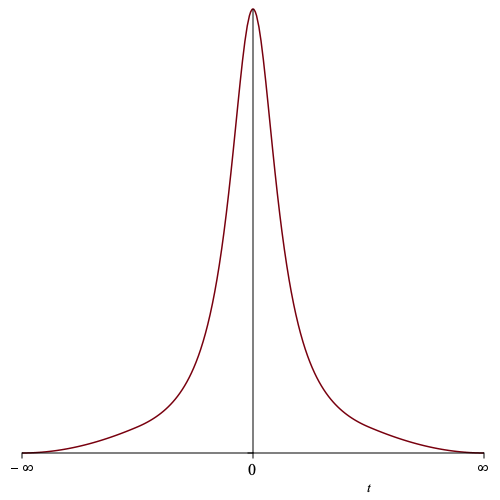
Maple tells us that the antiderivative is $\tan^{-1}t$. (I have also used Maple for all these graphs.)

Once again, Lebesgue integration is the way to go, since the necessary machinery has not been set up for gauge integrals. The formal proof has the same structure as in the previous example. We verify the antiderivative, show continuity of the integrand and also show the integrand to be nonnegative. Finally, we apply the FTC to obtain the two conclusions.

lemma
  defines "f' ≡ λt. 1 / (t⇧2+1)"
  shows
    "set_integrable lborel (einterval (-∞) ∞) f'"
    "(LBINT t=-∞..∞. f' t) = pi"
proof -
  have "(arctan has_real_derivative f' t) (at t)" for t
    unfolding f'_def 
    by (rule derivative_eq_intros | force simp: divide_simps)+
  moreover
  have "isCont f' x" for x
    unfolding f'_def
    by (intro continuous_intros) (auto simp: add_nonneg_eq_0_iff) 
  moreover
  have "((arctan ∘ real_of_ereal) ⤏ -pi/2) (at_right (-∞))"
       "((arctan ∘ real_of_ereal) ⤏ pi/2) (at_left ∞)"
    by (simp add: ereal_tendsto_simps1, real_asymp)+
  ultimately show "set_integrable lborel (einterval (-∞) ∞) f'"
    "interval_lebesgue_integral lborel (-∞) ∞ f' = pi"
    using interval_integral_FTC_nonneg [of "-∞" ∞ arctan]
    by (auto simp: f'_def)
qed

There are a couple of differences from the previous proof. We do not need an abbreviation for the antiderivative because it is simply arctan. But this proof features a local definition of the integrand as f', and we could have done something similar last time.

Integration of a sign-changing function

If you are unsure why a sign-changing function needs a different version of the FTC, consider that $\cos$ is both differentiable and continuous. Without the non-negative condition, the FTC would tell us that $\cos$ could be integrated over the whole real line, which is ridiculous.

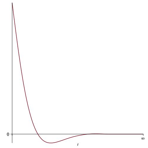
And so our final example is to integrate a damped sinusoid over the non-negative real numbers.

Here is the graph. It’s hard to see, but this function crosses the $x$-axis infinitely often.

Because its sign changes, the integration proof involves two steps:

1. Show that the integral exists. Since $\lvert e^{-t}\cos t\rvert \le e^{-t}$, we need to show that the latter function is integrable. It is non-negative, so we apply the previous version of the FTC.
2. We apply a signed version of the FTC to verify what the value of the integral actually is.

Let’s do the formal proof. We start with the theorem statement, including as before a local definition of the integrand.

lemma
  defines "f' ≡ λt. exp(-t) * cos(t)"
  shows  "set_integrable lborel (einterval 0 ∞) f'"
         "(LBINT t=0..∞. f' t) = 1/2"
proof -

The first result

Concerning step 1 above, we show that $e^{-t}$ is integrable. The proof relies on the FTC for non-negative functions, just as we’ve already. Our task this time is slightly simpler because we don’t care what the integral actually is. (It’s 1.) We can therefore ignore the second conclusion of interval_integral_FTC_nonneg and write the proof as follows:

  have "set_integrable lborel (einterval 0 ∞) (λt. exp(-t))"
  proof (rule interval_integral_FTC_nonneg)
    show "((λt. -exp(-t)) has_real_derivative exp(-t)) (at t)" for t
      by (rule derivative_eq_intros | force simp: field_simps)+
    have "(((λt. -exp (-t)) ∘ real_of_ereal) ⤏ -1) (at_right (ereal 0))"
      by (simp add: ereal_tendsto_simps1, real_asymp)
    then show "(((λt. -exp (-t)) ∘ real_of_ereal) ⤏ -1) (at_right 0)"
      by (simp add: zero_ereal_def)
    show "(((λt. - exp (- t)) ∘ real_of_ereal) ⤏ 0) (at_left ∞)"
      by (simp add: ereal_tendsto_simps1, real_asymp)
  qed auto

Setting this fact aside, we prove a necessary technical condition: that the integrand is a measurable function on the closed interval $[0,\infty]$.

  moreover have "set_borel_measurable lborel (einterval 0 ∞) f'"
    using borel_measurable_continuous_on_indicator 
    by (simp add: f'_def set_borel_measurable_def)

We store this fact as well, and then prove that the integrand is absolutely bounded by $e^{-t}$.

  moreover have "⋀t. ¦f' t¦ ≤ exp(-t)"
    by (simp add: f'_def abs_mult)

Combining the facts proved above, we find that f' is indeed integrable over $[0,\infty]$. This is the first conclusion of the theorem, but we also label it because it’s needed to prove the second conclusion.

  ultimately show *: "set_integrable lborel (einterval 0 ∞) f'"
    by (metis (mono_tags, lifting) abs_exp_cancel always_eventually
        real_norm_def set_integrable_bound set_integrable_bound)

The second result

Now we turn to step 2. We insert a local definition of the antiderivative, which happens to be \(e^{-t}\frac{\sin t - \cos t}{2}\). To prove the second conclusion, we express the integral as the difference between two values at the endpoints and apply the more general version of the FTC.

  define f where "f ≡ λt::real. exp(-t) * (sin(t) - cos(t)) / 2"
  have "(LBINT t=0..∞. f' t) = 0 - (- 1/2)"
  proof (intro interval_integral_FTC_integrable)

The next steps should be familiar by now. For an arbitrary real number t, we verify the antiderivative by differentiation and prove the integrand to be continuous.

    fix t
    show "(f has_vector_derivative f' t) (at t)"
      unfolding f_def f'_def has_real_derivative_iff_has_vector_derivative [symmetric]
      by (rule derivative_eq_intros | force simp: field_simps)+
    show "isCont f' t"
      unfolding f'_def by (intro continuous_intros)

The FTC requires us to verify the values attained by the antiderivative at the endpoints. Which we do using the techniques we’ve seen before, in particular, a couple of awkward tricks needed because everything has to be proved in terms of the extended real numbers.

  next
    have "((f ∘ real_of_ereal) ⤏ -1/2) (at_right (ereal 0))"
      by (simp add: ereal_tendsto_simps1 f_def, real_asymp)
    then show "((f ∘ real_of_ereal) ⤏ -1/2) (at_right 0)"
      by (simp add: zero_ereal_def)
    show "((f ∘ real_of_ereal) ⤏ 0) (at_left ∞)"
      by (simp add: ereal_tendsto_simps1 f_def, real_asymp)

Now auto (given the first result, namely *) wraps up the proof.

  qed (use * in auto)
  then show "(LBINT t=0..∞. f' t) = 1/2"
    by simp
qed

A few concluding remarks

As we have seen, an Isabelle theorem declaration can have multiple conclusions. In the case of interval_integral_FTC_nonneg, it makes sense because both conclusions depend on the same premises and much of the same reasoning. In the last example, I did this simply for the sake of uniformity. In the case of gauge integrals, Isabelle provides has_integral to express that the integral exists and has the given value. Somewhat similarly, has_bochner_integral refers to Lebesgue integrals, but it is a bit clunky for integrating over the real line.

The Isabelle theory file formalising the examples in this and the previous post are online.